Planes#
All Lentil planes are derived from the Plane class. This base class defines
the interface to represent any discretely sampled plane in an optical model.
Planes typically have some influence on the propagation of a wavefront though
this is not strictly required and models may use dummy or reference planes
as needed.
Lentil provides several general planes that are the building blocks for most optical models:
The
Planebase class provides the core logic for representing and working with discretely sampled planes in an optical model.The
Pupilplane provides a convenient way to represent a pupil plane in an optical system. There is nothing particularly special about pupil planes, they merely provide a convenient location (mathematically-speaking) to enforce limiting apertures or stops and include optical aberrations. More detailed discussion of pupil planes is available in [1].The
Imageplane provides a location where the image formed by an optical system may be manipulated or viewed.
In addition, several “utility” planes are provided. These planes do not represent physical components of an optical system, but are used to implement commonly encountered optical effects:
The
Tiltplane is used to represent wavefront tilt in terms of radians of x and y tilt.The
Rotateplane rotates a wavefront by an arbitrary angle.The
Flipplane flips a wavefront about its x, y, or both x and y axes.
Plane#
Lentil’s Plane class represents a discretely sampled plane in an optical
model. Planes have attributes for representing the sampled complex amplitude
of the plane as well as additional metadata that may influence how a
propagating wavefront interacts with the plane. A plane is defined by the
following parameters:
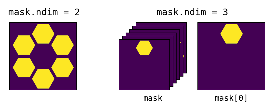
amplitude- Defines the relative electric field amplitude transmission through the planeopd- Defines the optical path difference that a wavefront experiences when propagating through the planemask- Defines the binary mask over which the plane data is valid. If mask is 2-dimensional, the plane is assumed to be monolithic. If mask is 3-dimensional, the plane is assumed to be segmented with the individual segment masks inserted along the first dimension. If mask is not provided, it is automatically created as needed from the nonzero values inamplitude.
pixelscale- Defines the physical sampling of the above attributes. A simple example of how to calculate the pixelscale for a discretely sampled circular aperture is given below: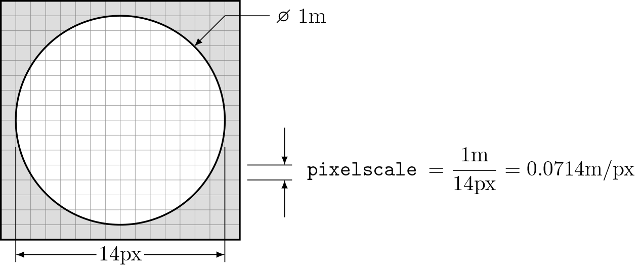
Note
All Plane attributes have sensible default values that have no effect on propagations when not specified.
Create a new Plane with
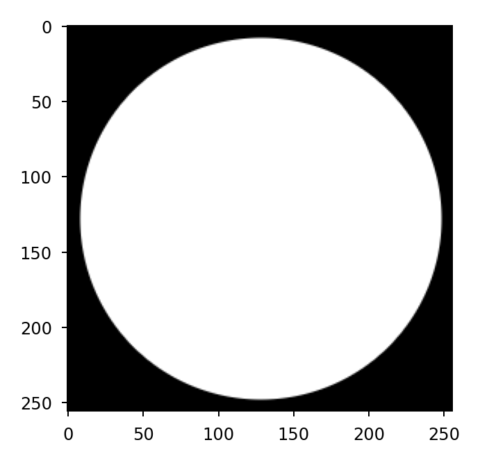
>>> p = lentil.Plane(amplitude=lentil.circle((256,256), 120))
>>> plt.imshow(p.amplitude, cmap='gray')
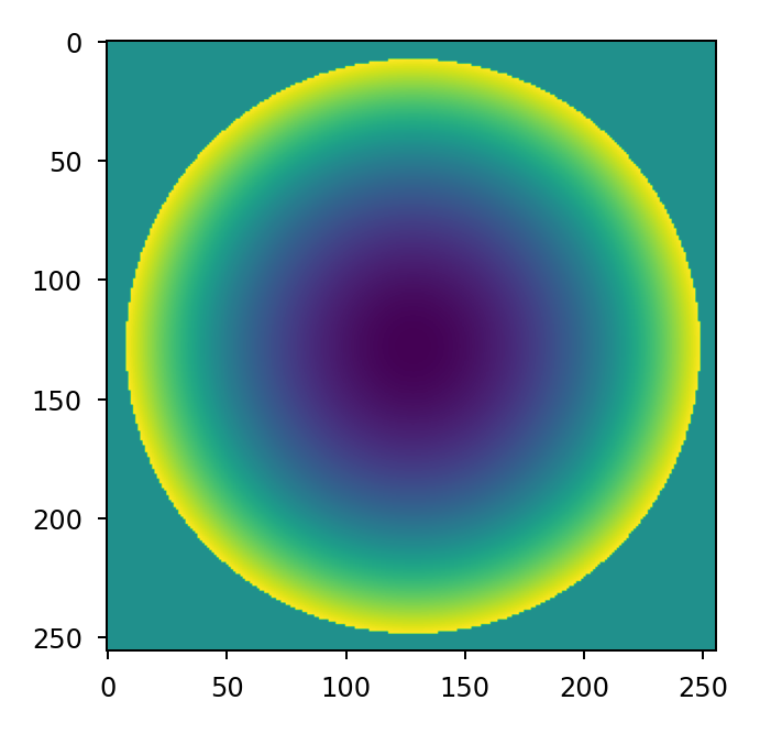
Once a Plane is defined, its attributes can be modified at any time:
>>> p = lentil.Plane(amplitude=lentil.circle((256,256), 120))
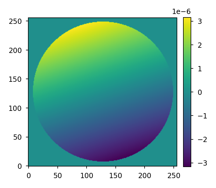
>>> p.opd = 2e-6 * lentil.zernike(p.mask, index=4)
>>> plt.imshow(p.opd, cmap=opd_cmap)
Resampling or rescaling a Plane#
It is possible to resample a plane using either the
resample() or rescale() methods. Both
methods use intrepolation to resample the amplitude, opd, and mask attributes
and readjust the pixelscale attribute as necessary.
Creating a frozen copy of a Plane#
Some custom Planes like the
tip/tilt mirror defined below
implement custom opd functionality that computes a
dynamic OPD value on the fly. When opd needs to be
repeatedly accessed (for example, when performing a
broadband propagation) and
is expensive to calculate, it can be beneficial to operate on a
copy of the plane where its opd attribute has
been “frozen”. This is easily accomplished using the
freeze() method:
>>> tt = TipTiltMirror()
>>> tt.x = [1e-6, 3e-6]
>>> ttf = tt.freeze()
By default, only the opd attribute is frozen, but
it’s possible to freeze any other attribute by passing its name to
freeze():
>>> ttf = tt.freeze('other_attr')
ptype#
A plane’s type (ptype) defines how it interacts with a
Wavefront. When a wavefront interacts with a plane, it inherits the plane’s
ptype. Plane type is set automatically and unexpected behavior may
occur if it is changed.
Lentil planes support the following ptypes:
ptype |
Planes with this type |
|---|---|
|
|
|
|
|
|
|
|
|
The rules defining when a wavefront is allowed to interact with a plane based
on ptype are described
here.
Pupil#
Lentil’s Pupil class provides a convenient way to represent a generalized
pupil function. Pupil planes behave exactly like Plane objects but
introduce an implied spherical phase term defined by the
focal_length attribute. The spherical phase term is
opaque to the user but is given by
where \(f\) is the focal length and \(x\) and \(y\) are pupil plane coordinates.
A pupil is defined by the following required parameters:
focal_length- The effective focal length (in meters) represented by the pupilpixelscale- Defines the physical sampling of each pixel in the discretely sampled attributes described below
Discreetly sampled pupil attributes can also be specified:
amplitude- Defines the relative electric field amplitude transmission through the pupilopd- Defines the optical path difference that a wavefront experiences when propagating through the pupil.mask- Defines the binary mask over which the pupil data is valid. If mask is 2-dimensional, the pupil is assumed to be monolithic. If mask is 3-dimensional, the pupil is assumed to be segmented with the segment masks allocated along the first dimension. If mask is not provided, it is automatically created as needed from the nonzero values inamplitude.
Note
All optional Pupil attributes have sensible default values that have no effect on propagations when not defined.
Create a pupil with:
>>> p = lentil.Pupil(focal_length=10, pixelscale=1/100, amplitude=1, opd=0)
Image#
Lentil’s Image plane is used to either manipulate or view a wavefront at an
image plane in an optical system. An image plane does not have any required
parameters although any of the following can be specified:
pixelscale- Defines the physical sampling of each pixel in the image plane. If not provided, the sampling will be automatically selected to ensure the results are at least Nyquist sampled.shape- Defines the shape of the image plane. If not provided, the image plane will grow as necessary to capture all data.amplitude- Definers the relative electric field amplitude transmission through the image plane.opd- Defines the optical path difference that a wavefront experiences when propagating through the image plane.
Tilt#
The Tilt plane provides a mechanism for directly specifying
wavefront tilt outside of the context of a discretely sampled Plane object.
Tilt is most useful for representing global tilt in an
optical system (for example, due to a pointing error).
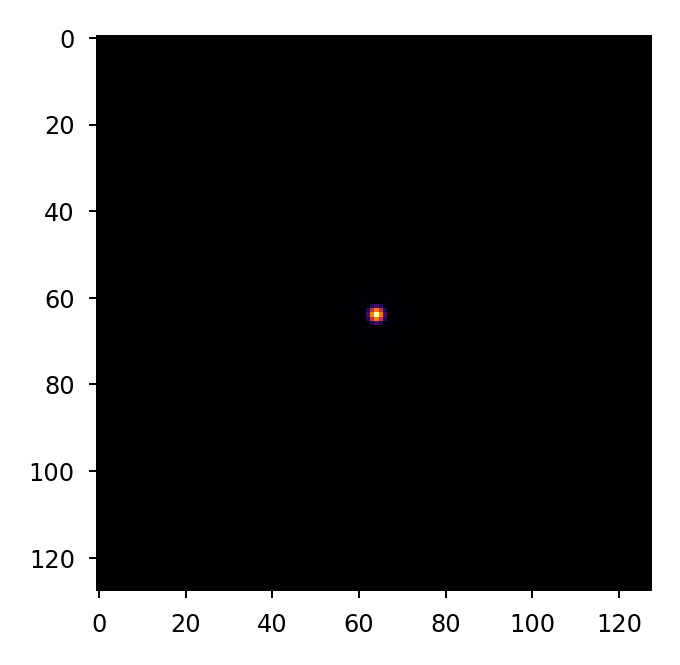
Given the following Pupil plane:
>>> pupil = lentil.Pupil(amplitude=lentil.circle((256, 256), 120),
...                      focal_length=10, pixelscale=1/250)
>>> w = lentil.Wavefront(650e-9)
>>> w *= pupil
>>> w = lentil.propagate_dft(w, pixelscale=5e-6, shape=(64,64), oversample=2)
>>> plt.imshow(w.intensity, cmap='inferno')
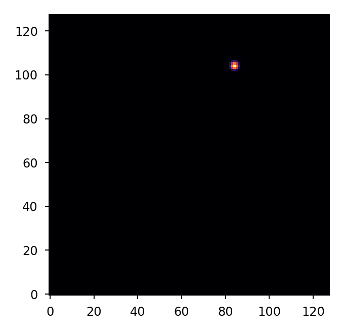
It is simple to see the effect of introducing a tilted wavefront into the system:
>>> pupil = lentil.Pupil(amplitude=lentil.circle((256, 256), 120),
...                      focal_length=10, pixelscale=1/250)
>>> tilt = lentil.Tilt(x=10e-6, y=-5e-6)
>>> w = lentil.Wavefront(650e-9)
>>> w *= pupil
>>> w *= tilt
>>> w = lentil.propagate_dft(w, pixelscale=5e-6, shape=(64,64), oversample=2)
>>> plt.imshow(w.intensity, origin='lower', cmap='inferno')
Note
Notice the use of origin='lower' in the plot above. For an explanation,
see the note here.
Dispersive planes#
DispersiveTilt#
Grism#
Warning
Grism is deprecated and will be removed in a future
version. Use DispersiveTilt instead.
A grism is a combination of a diffraction grating and a prism that creates a dispersed spectrum normal to the optical axis. This is in contrast to a single grating or prism, which creates a dispersed spectrum at some angle that deviates from the optical axis. Grisms are most commonly used to create dispersed spectra for slitless spectroscopy or to create interference fringes for dispersed fringe sensing.
Lentil’s Grism plane provides a straightforward mechanism for
efficiently modeling a grism.
Active optics and deformable mirrors#
Active optics and deformable mirrors are easily represented by defining an OPD
that depends on some parameterized state. Because there is no standard
architecture for these types of optical elements, Lentil does not provide a
concrete implementation. Instead, a custom subclass of either Plane or
Pupil should be defined. The exact implementation details will vary by
application, but a simple example of a tip-tilt mirror where the plane’s OPD
is computed dynamically based on the state x is provided below.
import lentil
import numpy as np

class TipTiltMirror(lentil.Plane):

    def __init__(self):
        self.amplitude = lentil.circle((256,256),120)

        self.x = np.zeros(2)

        # Note that we set normalize=False so that each mode spans [-1, 1]
        # and then multiply by 0.5 so that each mode has peak-valley = 1
        self._infl_fn = 0.5 * lentil.zernike_basis(mask=self.amplitude,
                                                   modes=[2,3],
                                                   normalize=False)

    @property
    def opd(self):
        return np.einsum('ijk,i->jk', self._infl_fn, self.x)
>>> tt = TipTiltMirror()
>>> tt.x = [1e-6, 3e-6]
>>> plt.imshow(tt.opd, cmap=opd_cmap)
>>> plt.colorbar()
