Utilities#
Shapes#
Loupe provides functions for drawing several useful shapes inside Numpy arrays.
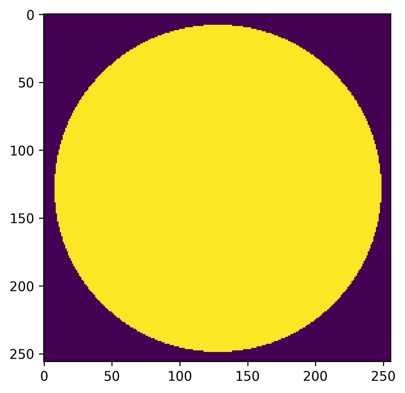
Circles#
To draw a filled circle with a hard edge, use circlemask():
>>> import matplotlib.pyplot as plt
>>> import loupe
>>> c = loupe.circlemask(shape=(256, 256), radius=120)
>>> plt.imshow(c)
To draw a filled circle with an antialiased edge, use circle():
>>> ca = loupe.circle(shape=(256, 256), radius=120)
>>> plt.imshow(ca)

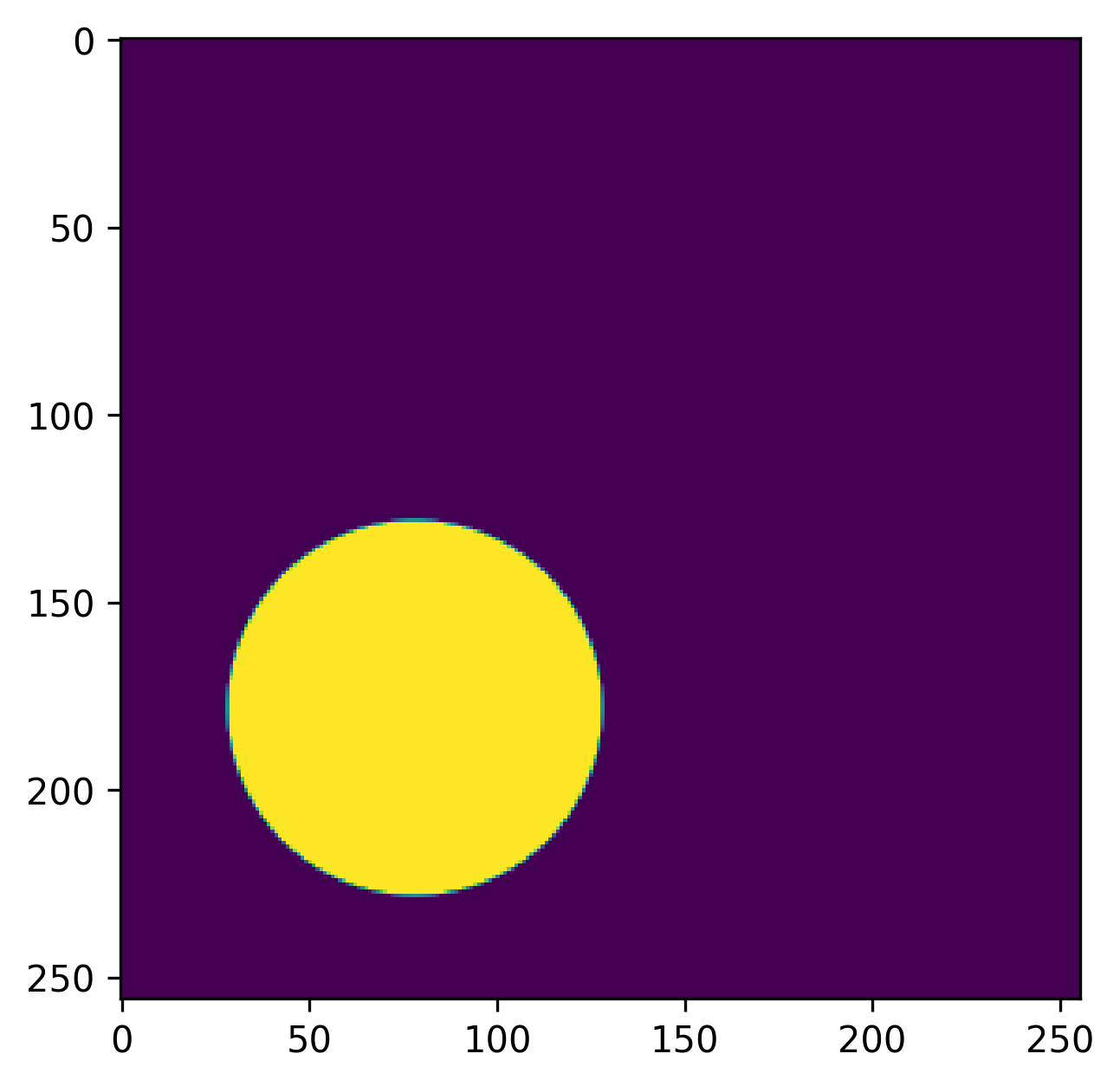
Note that both circle and circlemask accept a shift argument, which defines a desired row, col shift of the center of the circle:
>>> cs = loupe.circle(shape=(256, 256), radius=50, shift=(50, -50))
>>> plt.imshow(cs)
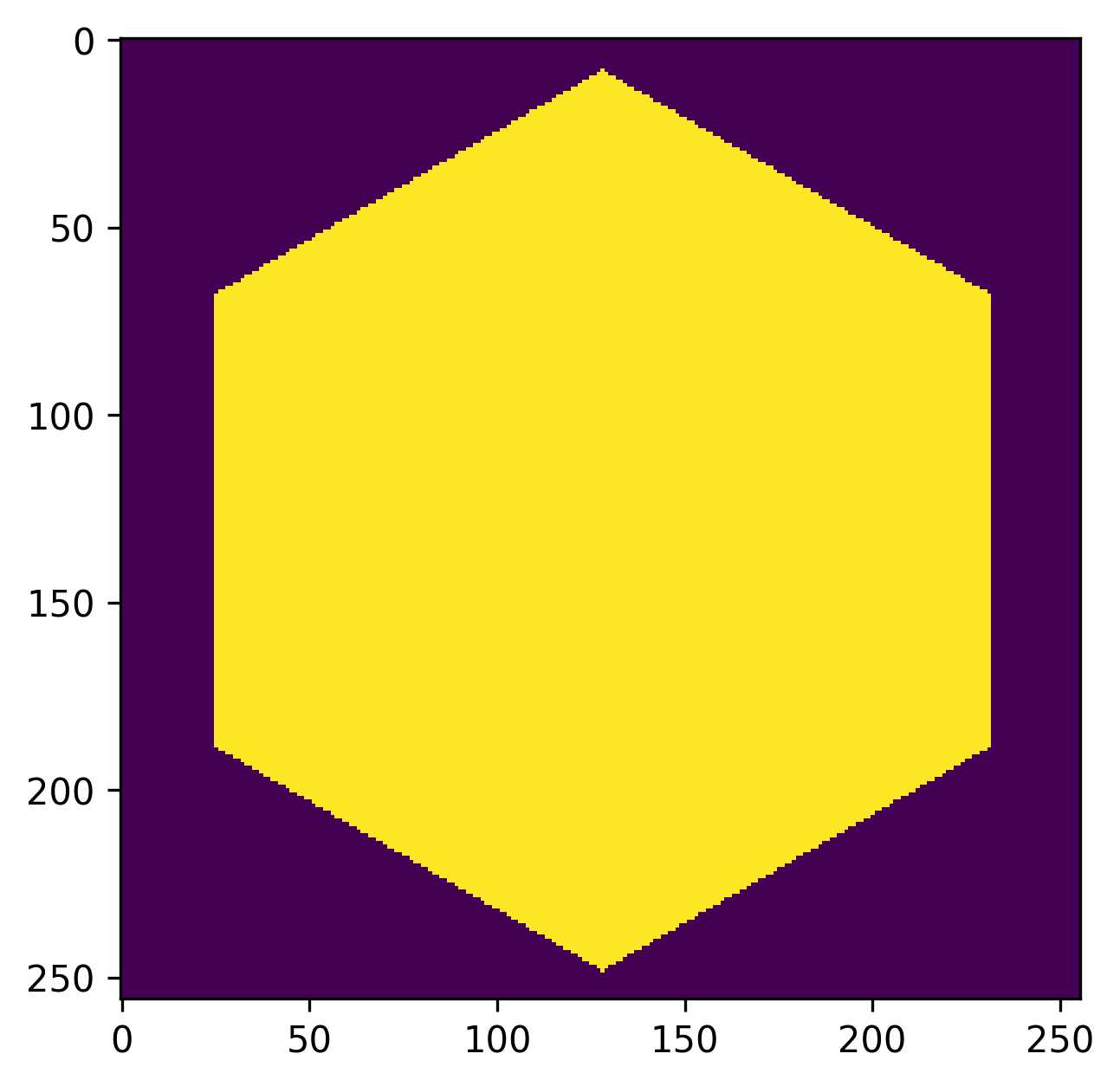
Hexagons#
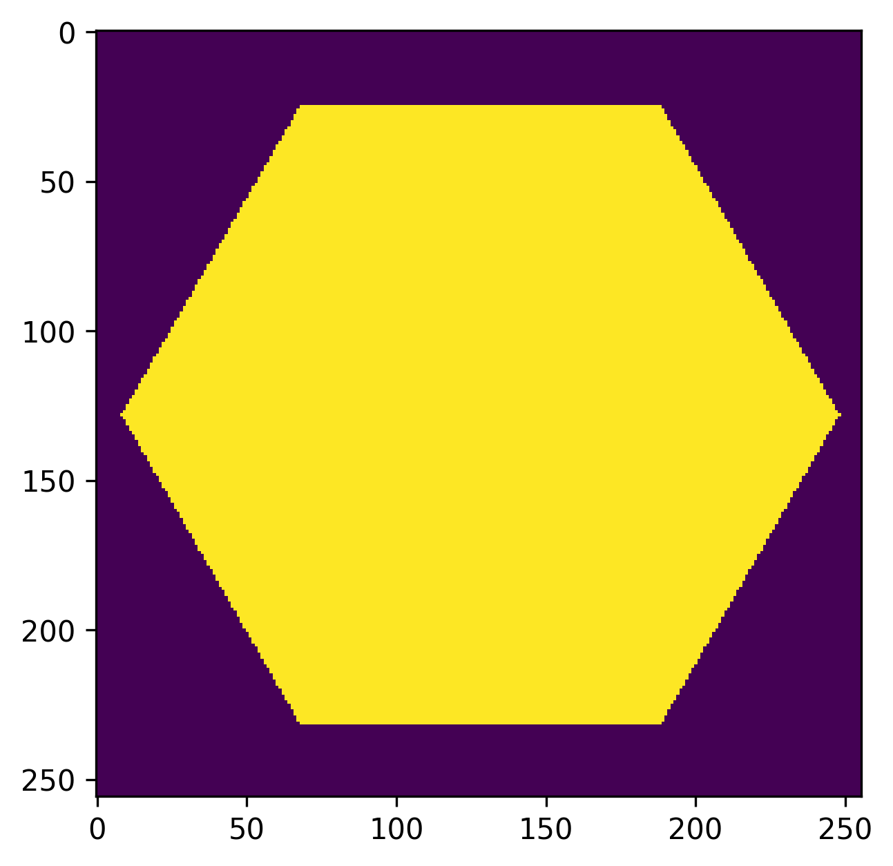
To draw a filled hexagon, use hexagon():
>>> import matplotlib.pyplot as plt
>>> import loupe
>>> h = loupe.hexagon(shape=(256, 256), radius=120)
>>> plt.imshow(h)
Note that the default orientation has orients the hexagon so that the pointy
ends are along the top and bottom of the shape. Passing rotate=True
rotates the hexagon 90 degrees so that the flat sides are along the top and
bottom of the shape:
>>> hr = loupe.hexagon(shape=(256, 256), radius=120, rotate=True)
>>> plt.imshow(hr)
Slits#
To draw a horizontal slit, use slit():
>>> import matplotlib.pyplot as plt
>>> import loupe
>>> s = loupe.slit(shape=(256, 256), width=11)
>>> plt.imshow(s)
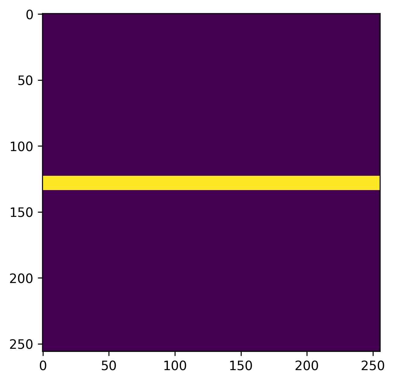
Image processing#
Computing image centroids#
The centroid of an image is the arithmetic mean position of all pixels in the
image. To compute the centroid of an image (or array), use
centroid():
>>> import numpy as np
>>> import loupe
>>> img = np.zeros((3,3))
>>> img[1,1] = 1
>>> loupe.centroid(img)
(1.0, 1.0)
Translating images#
To translate an image by an arbitrary number of pixels in row and column, use
shift():
>>> import numpy as np
>>> import loupe
>>> img = np.zeros((3,3))
>>> img[2,2] = 1
>>> img_shifted = loupe.shift(img, shift=(-1, -1))
>>> img_shifted
array([[ 0.00000000e+00, -7.40148683e-17, -2.46716228e-17],
       [-1.16747372e-16,  1.00000000e+00,  2.14548192e-16],
       [-3.12823642e-17,  2.22044605e-16, -4.18468327e-17]])
Note that because the shift is performed in the frequency domain, the shifts are not constrained to be integers.
Image registration#
To compute the relative shift between two images of the same size, use
register(). This function uses the cross-correlation of the two
inputs to compute the integer shift between the two images, and then
optionally computes an oversampled cross-correlation over a smaller window
using the DFT to compute the remaining subpixel shift to an arbitrary
precision.
For example, we’ll compute the shift between an image arr and a reference
image ref. For this example, arr is known to be shifted by
(-24.8, 36.2) pixels relative to ref:
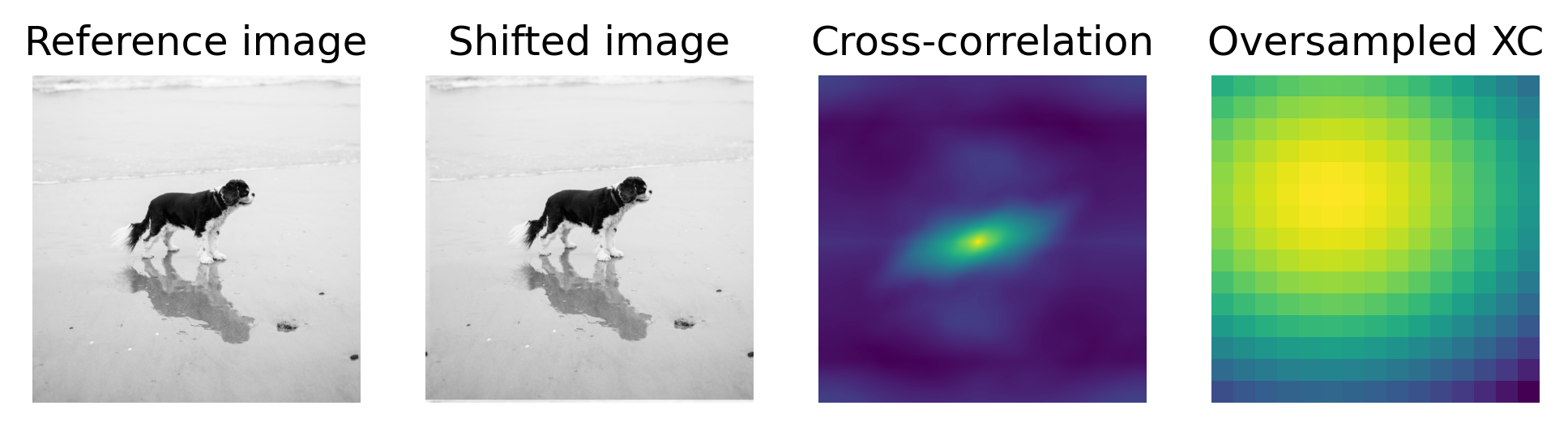
>>> import loupe
>>> loupe.register(arr, ref, oversample=10)
(24.8, -36.2)
Zernike polynomials#
Loupe providea a number of utilities for working with Zernike polynomials. Methods are provided for creating, fitting, and removing Zernikes.
Note
Lentil uses the Noll indexing scheme for defining Zernike polynomials [1].
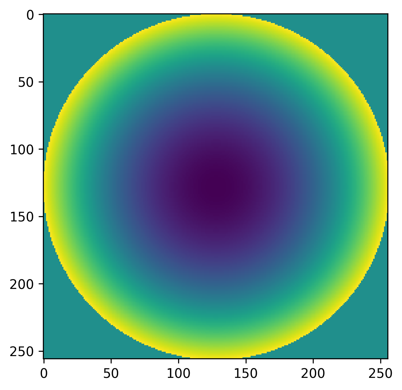
Constructing Zernikes#
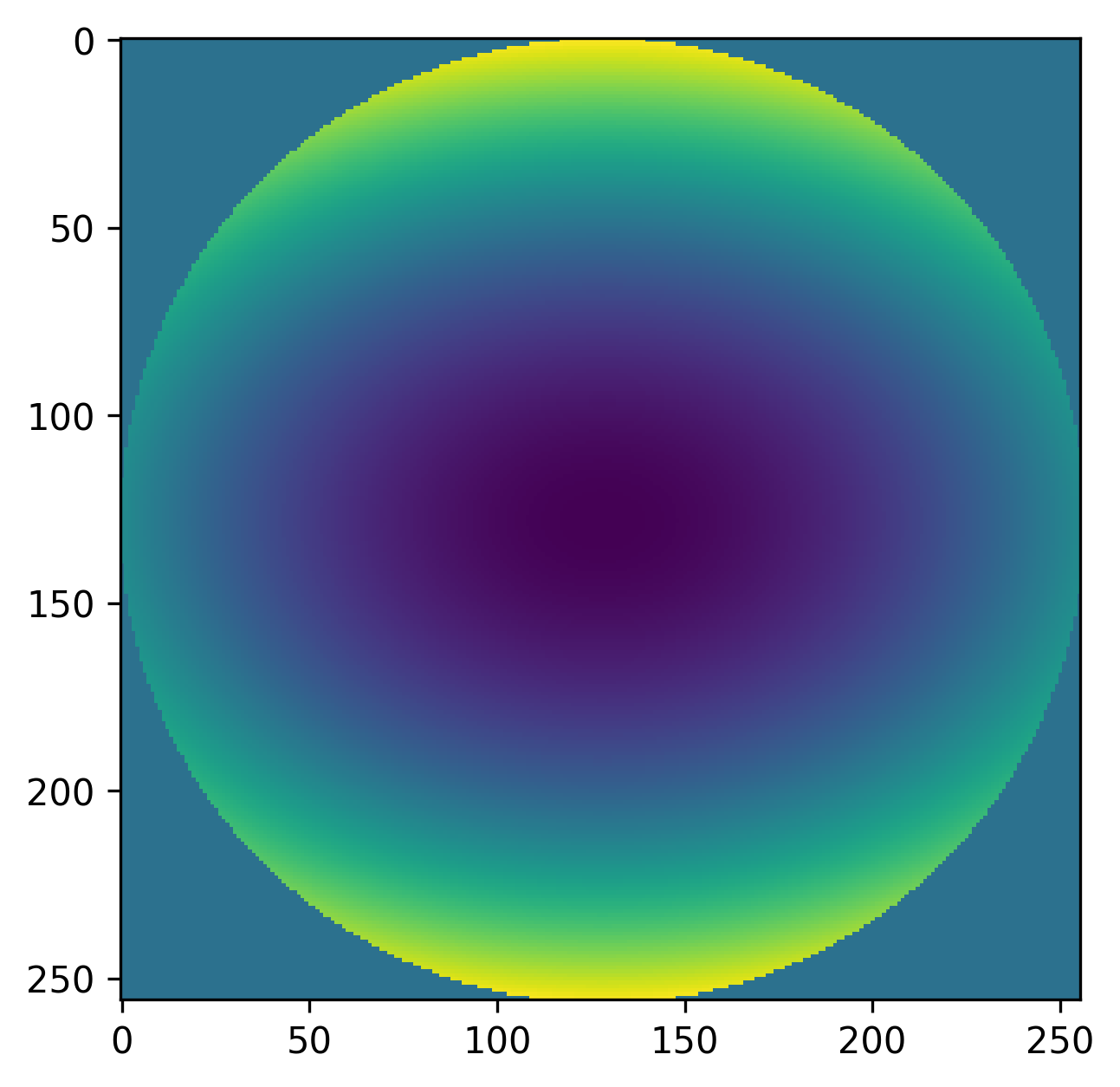
Single Zernike maps are created with the loupe.zernike() function. For
example, we can create a map representing 100 units of focus (Z4) over a
circular mask with:
>>> import matplotlib.pyplot as plt
>>> import loupe
>>> mask = loupe.circlemask((256,256), 128)
>>> z4 = 100 * loupe.zernike(mask, index=4)
>>> plt.imshow(z4)
Any combination of Zernike polynomials can be created by providing a list of
coefficients to the loupe.zernike_compose() function. For example, we
can represent 200 units of focus and -100 units of astigmatism as:
>>> import matplotlib.pyplot as plt
>>> import loupe
>>> mask = loupe.circlemask((256,256), 128)
>>> coefficients = [0, 0, 0, 200, 0, -100]
>>> z = loupe.zernike_compose(mask, coefficients)
>>> plt.imshow(z)
Note that the coefficients list is ordered according to the Noll indexing scheme so the first entry in the list represents piston (Z1), the second represents, tilt (Z2), and so on.
Zernike polynomials are commonly used as a basis set for fitting complex
complex shapes over a circular mask. The zernike_basis() function
provides a simple interface for creating such a basis set. Here, we’ll
construct a basis gconsisting of focus and astigmatism (Z4-Z6):
>>> import matplotlib.pyplot as plt
>>> import loupe
>>> mask = loupe.circlemask((256,256), 128)
>>> basis = loupe.zernike_basis(mask, modes=(4,6))
Fitting Zernikes#
Normalization#
Each of Loupe’s Zernike functions accept a normalize parameter. If normalize
is False (the default), the raw Zernike mode is returned. Each mode will approximately
span [-1 1] although this shouldn’t be relied upon because of the discrete sampling of
the result. If normalize is true, the Zernike mode will be normalized so that its
standard deviation equals 1 (over the supplied mask).
Normalization becomes important when trying to achieve a specific error magnitude,
whether it be in terms of RMS or peak to valley errors. To acihieve a specific error in terms
of RMS, Zernike modes should be computed with normalize=True before multiplying by
the error magnitude:
>>> import loupe
>>> import numpy as np
>>> mask = loupe.circlemask((256,256), 128)
>>> z4 = 100 * loupe.zernike(mask, mode=4, normalize=True)
>>> np.std(z4[np.nonzero(z4)])
99.86295346152438
To achieve a specific error in terms of peak to valley, Zernike modes should be computed and normalized separately. The separate normalization step should be performed to ensure the discretely sampled mode spans [-0.5 0.5] before multiplying by the error magnitude:
>>> import loupe
>>> import numpy as np
>>> mask = loupe.circlemask((256,256), 128)
>>> z4 = loupe.zernike(mask, mode=4)
>>> z4 /= np.max(z4) - np.min(z4)
>>> z4 *= 100
>>> np.max(z4) - np.min(z4)
100
Defining custom coordinates#
By default, all of Loupe’s Zernike functions place the center of the coordinate system
at the centroid of the supplied mask with its axes aligned to the Cartesian coordinate
system. This works as expected for the vast majority of
needs, but in some cases it may be desirable to manually define the coordinate system.
This is accomplished by using loupe.zernike_coordinates() to compute rho and
theta, and providing these definitions to the appropriate Zernike function. For
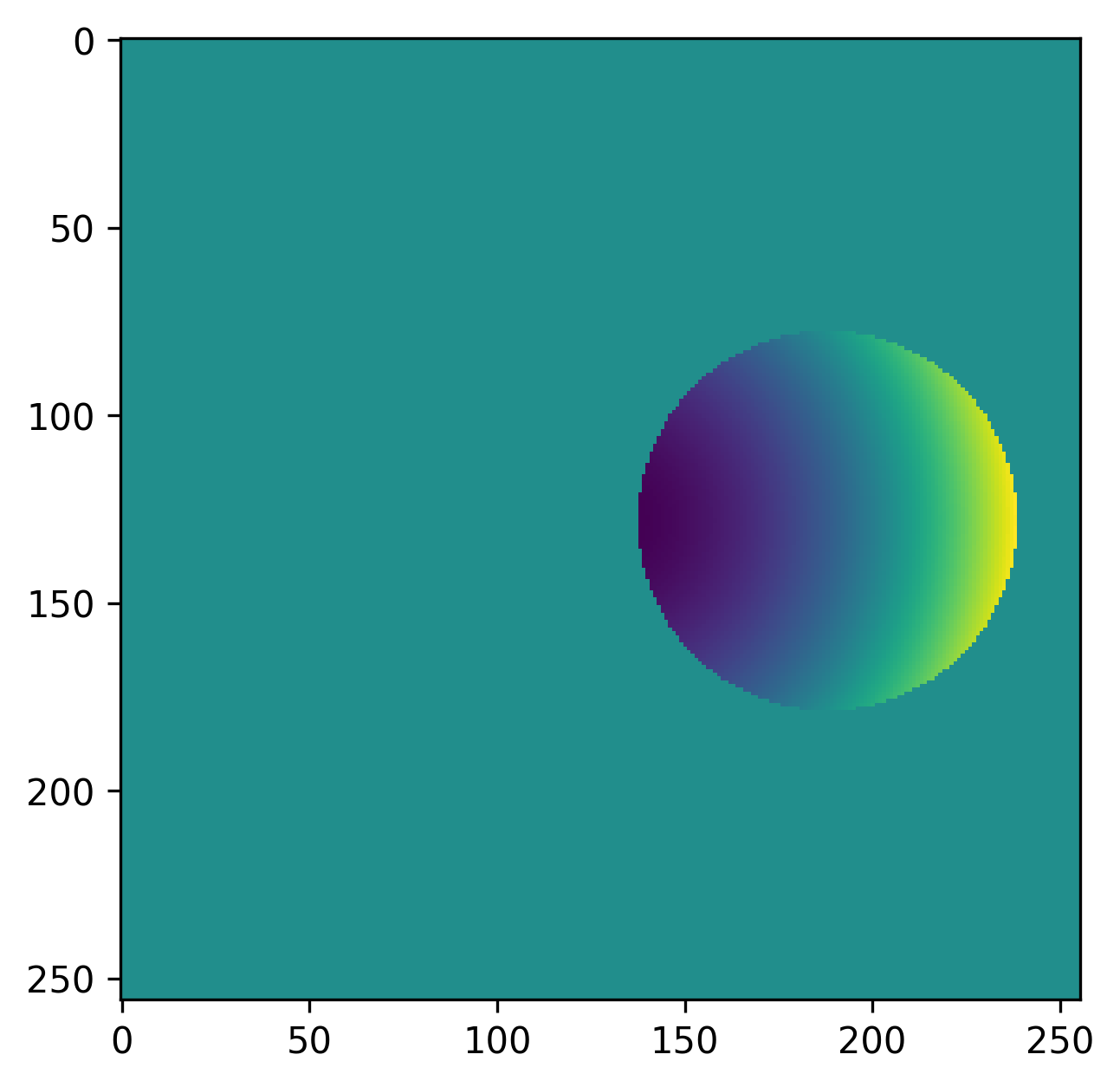
example, if we have an off-centered mask but wish to construct Zernikes relative to
the center of the defined array:
>>> import matplotlib.pyplot as plt
>>> import loupe
>>> mask = loupe.circlemask((256,256), radius=50, shift=(0,60))
>>> rho, theta = loupe.zernike_coordinates(mask, shift=(0,0))
>>> z4 = loupe.zernike(mask, 4, rho=rho, theta=theta)
>>> plt.imshow(z4)
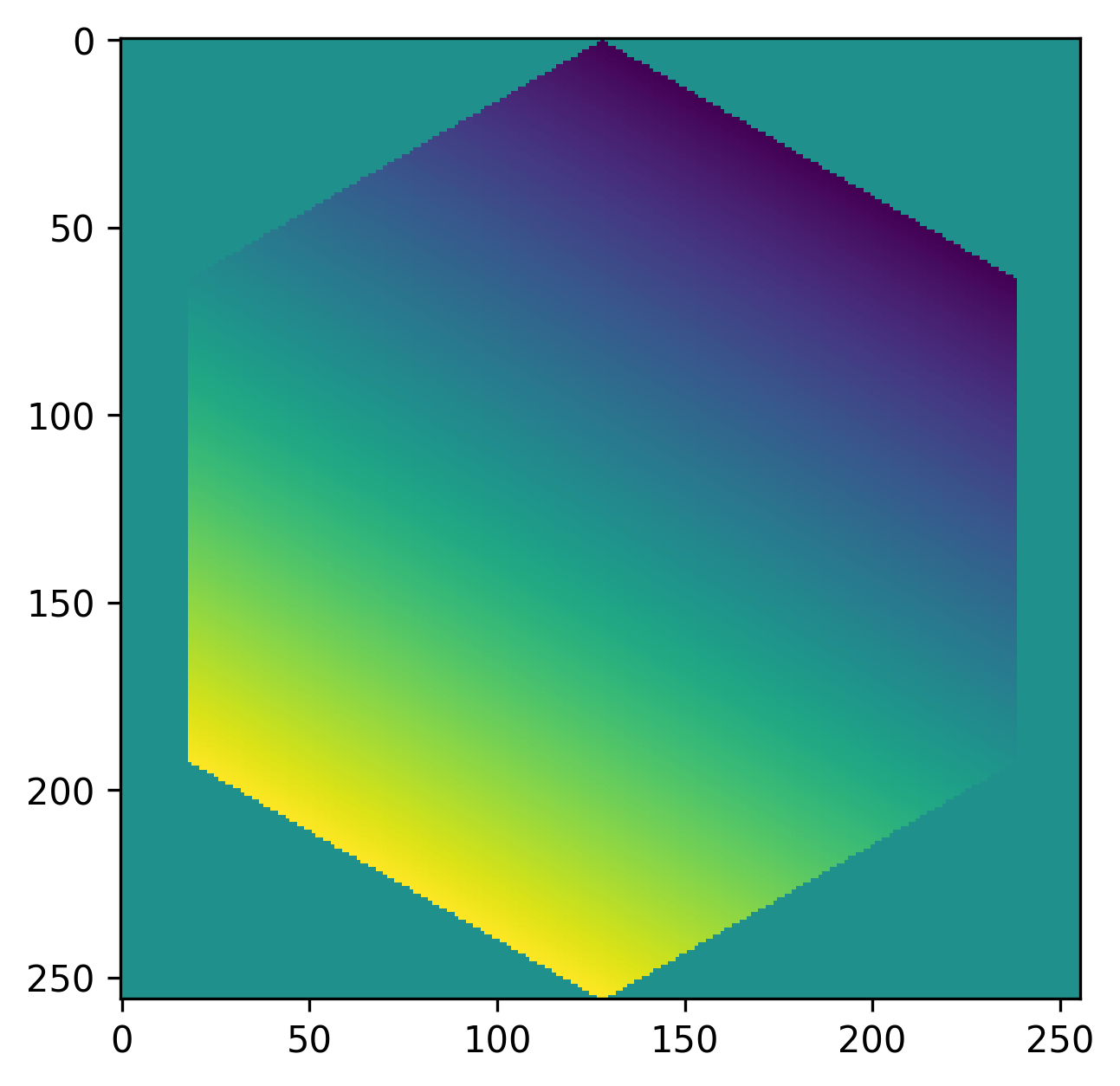
If we wish to align a tilt mode with one side of a hexagon:
>>> import matplotlib.pyplot as plt
>>> import loupe
>>> mask = loupe.hexagon((256,256), radius=128)
>>> rho, theta = loupe.zernike_coordinates(mask, shift=(0,0), rotate=60)
>>> z2 = loupe.zernike(mask, 2, rho=rho, theta=theta)
>>> plt.imshow(z2)