Array#

Introduction#

Loupe’s core object is the array. It is a multi-dimensional collection of elements of a single data type that are accessible using Python’s standard indexing notation. Loupe’s array interface is designed to be similar to Numpy’s ndarray with additional features for tracking array operations on a computational graph. Like in Numpy, Loupe’s array dimensions are called axes. The most commonly used array attributes are:

array.shape
The dimensions of the array. This is a tuple of integers indicating the size of the array in each dimension.
array.ndim
The number of axes (dimensions) of the array
array.size
The total number of elements of the array.
array.dtype
An object describing the type of the elements in the array.
array.data
The actual array data, stored as a Numpy array. Normally, we won’t need to use this attribute because we will access the elements in an array using indexing facilities.
array.requires_grad
A boolean indicating whether the gradient should be computed for the array.
array.grad
The gradient of the array, stored as a Numpy array.

Array creation#

There are several ways to create arrays. The simplest way is to pass a Python list or tuple to the array function:

>>> import loupe
>>> a = loupe.array([1,2,3])
>>> a
array([1., 2., 3.])

array transforms sequences of sequences into two-dimensional arrays, sequences of sequences of sequences into three-dimensional arrays, and so on:

>>> b = loupe.array([[1,2], [3,4]])
>>> b
array([[1., 2.],
       [3., 4.]])
>>> b.ndim
2

Loupe also provides several functions to create arrays with placeholder content. The function zeros creates an array full of zeros and the function ones creates an array full of ones:

>>> loupe.zeros((2,3))
array([[0., 0., 0.],
       [0., 0., 0.]])
>>> loupe.ones(5)
array([1., 1., 1., 1., 1.])

Indexing#

Array indexing refers to any use of the square brackets ([]) to index array values.

Note

Most of the following examples show the use of indexing when referencing data in an array. The examples work just as well when assigning to an array.

Indexing one-dimensional arrays#

Indexing for a 1-D array is what one expects. It work exactly like that for other standard Python sequences. Indexing is 0-based, and accepts negative indices for indexing from the end of the array:

>>> a = loupe.array([1,2,3,4,5])
>>> a[2]
3
>>> a[-2]
4

Indexing multi-dimensional arrays#

Unlike lists and tuples, arrays support multidimensional indexing for multidimensional arrays. It is not necessary to separate each dimension’s index into its own set of square brackets:

>>> b = loupe.array([[1,2,3], [4,5,6]])
>>> b[1,2]
6

Note that if one indexes a multidimensional array with fewer indices than dimensions, one gets a subdimensional array. For example:

>>> b[1]
array([4., 5., 6.])

Slices#

Arrays can be sliced using Python’s slice notation. Note that in order to preserve algorithmic differentation capibility, slices are returned as new slice objects rather than views of the underlying data.

For a one-dimensional array:

>>> c = loupe.array([5,6,7,8,9])
>>> c[2:]
array([7., 8., 9.])

and for multi-dimensional arrays:

>>> d = loupe.array([[2,4,6], [8,10,12], [14,16,18]])
>>> d[:,1:]
array([[  4.,  6.],
       [ 10., 12.],
       [ 16., 18.]])

Data types#

Numpy interoperability#

Loupe’s array implements Numpy’s dispatch mechanism, meaning Loupe arrays can be used anywhere Numpy arrays can be used:

>>> import numpy as np
>>> e = loupe.array([1,2,3])
>>> np.std(e)
5.163977794943222
>>> import matplotlib.pyplot as plt
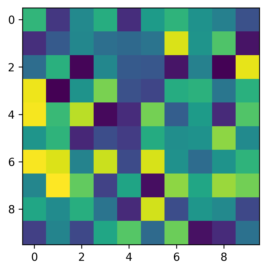
>>> f = loupe.rand(size=(10,10))
>>> plt.imshow(f)

This can be very useful for general analysis and plotting, but be aware that you will be leaving the Loupe ecosystem and dispatched operations are not tracked on Loupe’s computational graph.