Algorithmic differentiation

This page provides a brief overview of how Loupe’s algorithmic differentiation system (sometimes called automatic differentiation or autograd) works. It is not strictly necessary to understand this material to use Loupe, although a basic understanding will help you write simpler and more efficient models and may make debugging easier.

Computational graph

Internally, Loupe records all operations in a computational graph (or more specifically, a directed acyclic graph). The edges of this graph denote data dependencies. By tracing backward through a topological ordering of the graph, it is possible to automatically compute the gradients of input arrays using the chain rule. Loupe’s computational graph is defined dynamically as operations are applied to arrays and the results of other Loupe functions. For example:

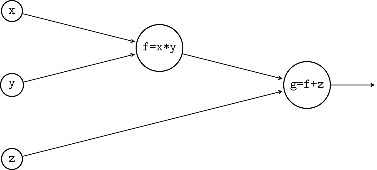
>>> x = loupe.array([1,2,3], requires_grad=True)
>>> y = loupe.array([4,5,6], requires_grad=True)
>>> f = x * y
>>> z = loupe.array(9, requires_grad=True)
>>> g = f + z
>>> g
array([13., 19., 27.])

When backward() is called, the gradients of the function inputs are computed and the results are accumulated in each array’s grad attribute:

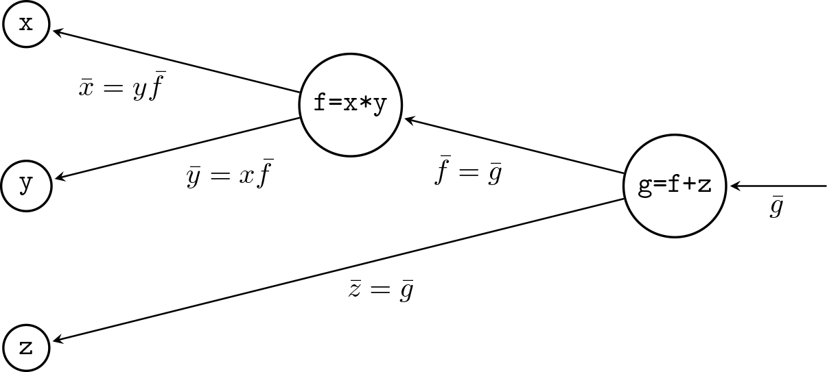
>>> g.backward(loupe.array([1,1,1]))
>>> x.grad
array([4., 5., 6.])
>>> y.grad
array([1., 2., 3.])
>>> z.grad
array(3.)

requires_grad

The array’s requires_grad attribute specifies whether the gradient should be accumulated for the array during a backwards pass. By setting requires_grad=True only for arrays whose gradients are required, unnecessary gradient calculations may be avoided.

Note that if a single input to an operation requires a gradient, the operation’s output will also require a gradient. Conversely, if none of an operation’s inputs require a gradient, the opeeration’s output also will not require a gradient.

When parameters are optimized using the optimize() function, the arrays requiring gradients are automatically marked and there is no need for the user to directly identify these arrays.