Lentil quickstart

Lentil is a Python library for modeling the imaging chain of an optical system. It was originally developed at NASA’s Jet Propulsion Lab by the Wavefront Sensing and Control group (383E) to provide an easy to use framework for simulating point spread functions of segmented aperture telescopes.

Lentil provides objects for defining optical planes and combining them to model diffraction and other imaging effects. It can be used to create models with varying levels of complexity - from simple prototypes to extremely high-fidelity models of ground or space telescopes.

Lentil uses one or more Plane objects to numericlly model an optical system. A Wavefront object representing a discretely sampled monochromatic plane wave is then propagated from plane to plane using one of the available numerical diffraction propagation routines. The resulting complex field can be visualized, analyzed, or further propagated through an optical model. Finally, Lentil includes a number of additional tools for representing common imaging artifacts, modeling focal plane arrays including many common noise sources, and working with radiometric quantities.

Below, we’ll walk through the steps to develop a very simple Lentil model of an imaging system with a single pupil and image plane. The imaging system has a 1 m diameter primary mirror, a secondary mirror obscuration of 0.33 m centered over the primary, a focal length of 20 m, and a focal plane with 5 um pixels.

First, we’ll import Lentil and matplotlib:

>>> import lentil
>>> import matplotlib.pyplot as plt

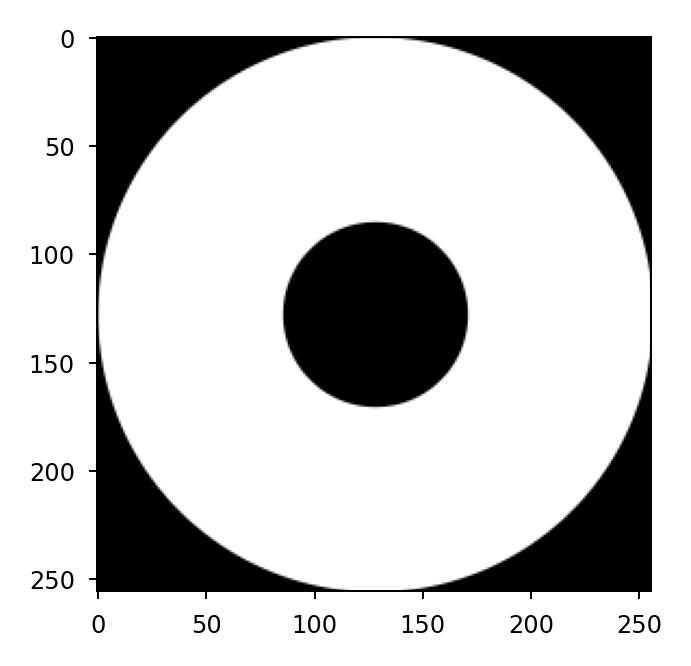
Now we can define the system amplitude and plot it:

>>> circ = lentil.circle(shape=(256, 256), radius=128)
>>> obsc = lentil.circle(shape=(256, 256), radius=128/3)
>>> amplitude = circ - obsc
>>> plt.imshow(amplitude, cmap='gray')

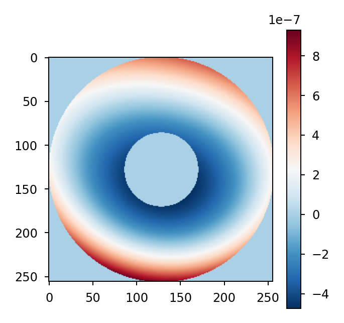
We’ll create some wavefront error using a small number of Zernike modes:

>>> coeffs = [0, 0, 0, 300e-9, 50e-9, -100e-9, 50e-9]
>>> opd = lentil.zernike_compose(mask=amplitude, coeffs=coeffs)
>>> plt.imshow(opd, cmap='RdBu_r')
>>> plt.colorbar()

Next we’ll define the system’s pupil plane. Note that the pixelscale attribute represents the physical sampling of each pixel in the pupil (in meters/pixel). Because our amplitude has a diameter of 256 pixels and the system diameter was specified as 1m, the pixelscale is 1/256.

>>> pupil = lentil.Pupil(amplitude=amplitude, opd=opd, diameter=1,
...                      focal_length=20, pixelscale=1/256)

Here we create a Wavefront and propagate it through the pupil plane we created above by multiplying the two objects together:

>>> wf = lentil.Wavefront(wavelength=650e-9)
>>> wf = wf * pupil

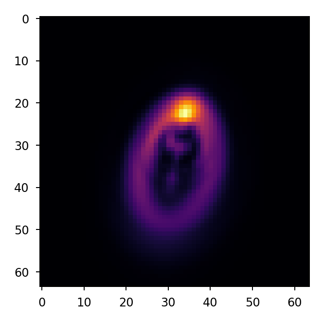
Now we can propagate the wavefront to the image plane using a discrete Fourier transform and plot the resulting image plane intensity:

>>> wf = lentil.propagate_dft(wf, shape=(64,64), pixelscale=5e-6, oversample=2)
>>> plt.imshow(wf.intensity, cmap='inferno')

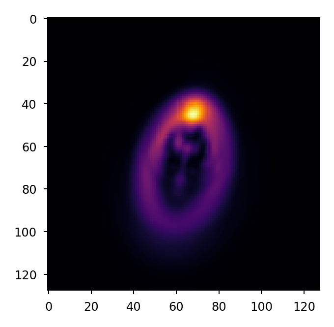
With a little extra code, we can perform a broadband propagation including many wavelengths in the simulation:

>>> img = 0
>>> for wl in np.arange(450e-9, 650e-9, 5e-9):
>>>     wf = lentil.Wavefront(wl)
>>>     wf = wf * pupil
>>>     wf = lentil.propagate_dft(wf, shape=(64,64), pixelscale=5e-6, oversample=2)
>>>     img += wf.intensity
>>> plt.imshow(img, cmap='inferno')

Finally, let’s convolve the oversampled image with the MTF of a square pixel and rebin the image to native detector sampling:

>>> img_det = lentil.detector.pixelate(img, oversample=2)
>>> plt.imshow(img_det, cmap='inferno')