Planes

Lentil represents optical systems using one or more planes that have some influence on a propagating wavefront. The following planes are the core building blocks of most models in Lentil:

• A Plane represents a discretely sampled optical plane at an arbitrary location in an optical system.

• A Pupil represents a discretely sampled pupil plane.

• An Image represents a discretely sampled image plane.

In addition, several “utility” planes are provided. These planes don’t represent physical components of an optical system, but are used to implement commonly encountered optical effects:

• The Tilt plane is used to represent wavefront tilt in terms x and y tilt (in radians).

Plane basics

Planes are described by a common set of attributes. The most commonly used attributes are

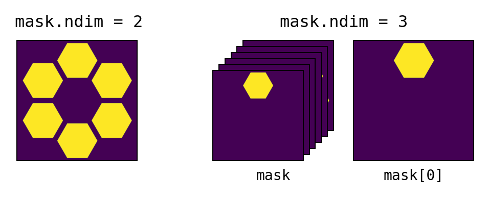
• amplitude - defines the electric field amplitude transmission through the plane

• opd - defines the optical path difference that a wavefront experiences when propagating through the plane

• mask - defines the binary mask over which the plane data is valid. If mask is 2-dimensional, the plane is assumed to be monolithic. If mask is 3-dimensional, the plane is assumed to be segmented with the individual segment masks provided along the first dimension. If mask is not provided, it is automatically created from the nonzero values in amplitude.

• pixelscale - defines the physical sampling of the above attributes. A simple example of how to calculate the pixelscale for a discretely sampled circular aperture is given below: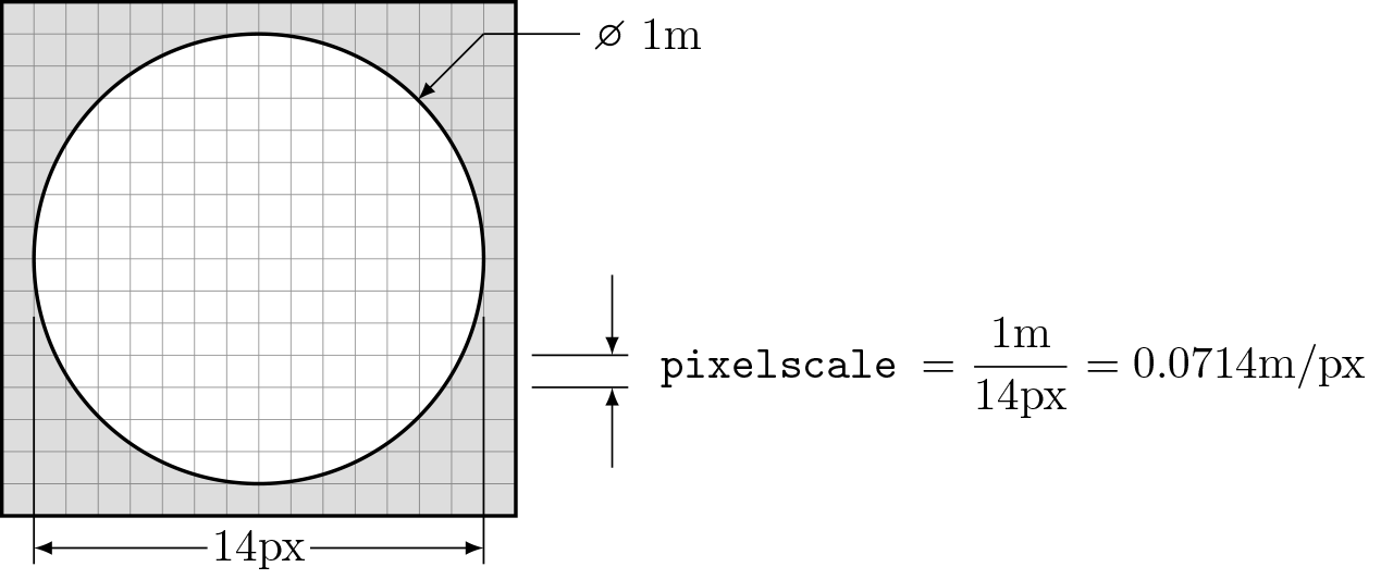

  

• ptype - specifies the plane type. Additional details are available in the sections describing How a plane affects a wavefront and Plane-wavefront multiplication rules

  Valid types are:

  ptype	Planes with this type
  none	Plane
  pupil	Pupil
  image	Image
  tilt	Tilt, DispersiveTilt
  transform	Rotate, Flip

Note

All Plane attributes have sensible default values that have no effect on propagations when not specified.

Plane creation

Create a new plane with

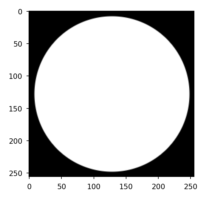
>>> p = lentil.Plane(amplitude=lentil.circle((256,256), 120))
>>> plt.imshow(p.amplitude, cmap='gray')

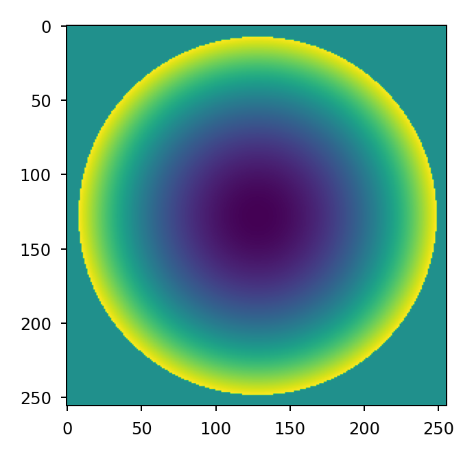
Once a plane is defined, its attributes can be modified at any time:

>>> p = lentil.Plane(amplitude=lentil.circle((256,256), 120))
>>> p.opd = 2e-6 * lentil.zernike(p.mask, index=4)
>>> plt.imshow(p.opd, cmap=opd_cmap)

Resampling and rescaling

It is possible to resample a plane using either the resample() or rescale() methods. Both methods use intrepolation to resample the amplitude, opd, and mask attributes and readjust the pixelscale attribute as necessary.

Pupil

Lentil’s Pupil class provides a convenient way to represent a generalized pupil function. Pupil planes behave exactly like plane objects but introduce an implied spherical phase term defined by the focal_length attribute. The spherical phase term is opaque to the user but is given by

\[\frac{1}{2f} \left(x^2 + y^2\right)\]

where \(f\) is the focal length and \(x\) and \(y\) are pupil plane coordinates.

A pupil is defined by the following required parameters:

• focal_length - The effective focal length (in meters) represented by the pupil

• pixelscale - Defines the physical sampling of each pixel in the discretely sampled attributes described below

Discreetly sampled pupil attributes can also be specified:

• ampltiude - Defines the relative electric field amplitude transmission through the pupil

• opd - Defines the optical path difference that a wavefront experiences when propagating through the pupil.

• mask - Defines the binary mask over which the pupil data is valid. If mask is 2-dimensional, the pupil is assumed to be monolithic. If mask is 3-dimensional, the pupil is assumed to be segmented with the segment masks allocated along the first dimension. If mask is not provided, it is automatically created as needed from the nonzero values in amplitude.

Note

All optional Pupil attributes have sensible default values that have no effect on propagations when not defined.

Create a pupil with:

>>> p = lentil.Pupil(focal_length=10, pixelscale=1/100, amplitude=1, opd=0)

Image

Lentil’s Image plane is used to either manipulate or view a wavefront at an image plane in an optical system. An image plane does not have any required parameters although any of the following can be specified:

• pixelscale - Defines the physical sampling of each pixel in the image plane. If not provided, the sampling will be automatically selected to ensure the results are at least Nyquist sampled.

• shape - Defines the shape of the image plane. If not provided, the image plane will grow as necessary to capture all data.

• amplitude - Definers the relative electric field amplitude transmission through the image plane.

• opd - Defines the optical path difference that a wavefront experiences when propagating through the image plane.

Tilt

The Tilt plane provides a mechanism for representing wavefront tilt in terms of angular rotations about the plane’s x and y-axes. This representation is separate and in addition to any tilt specified in a plane’s opd attribute. Tilt planes most useful for representing global tilt in an optical system (for example, due to a pointing error).

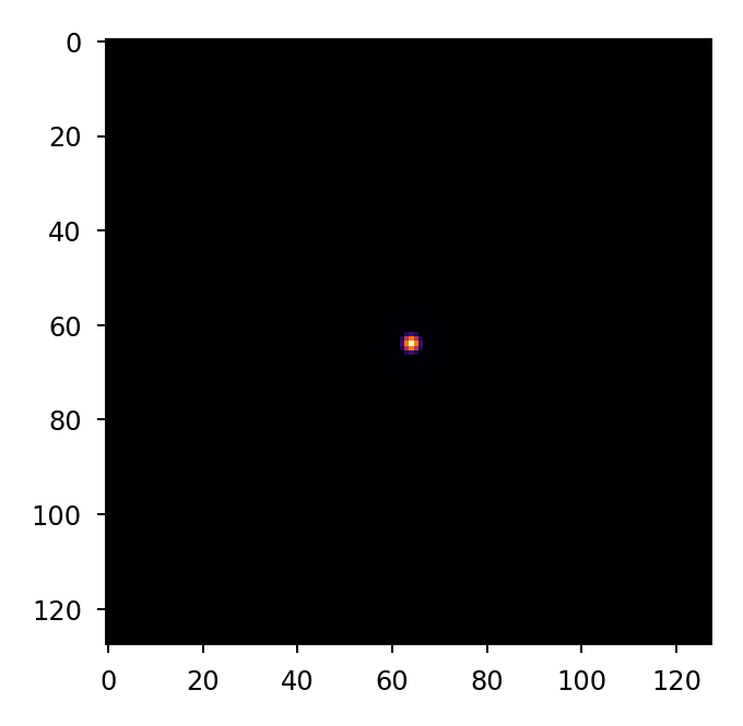
Given the following pupil plane:

>>> pupil = lentil.Pupil(amplitude=lentil.circle((256, 256), 120),
...                      focal_length=10, pixelscale=1/250)
>>> w = lentil.Wavefront(650e-9)
>>> w *= pupil
>>> w = lentil.propagate_dft(w, pixelscale=5e-6, shape=(64,64), oversample=2)
>>> plt.imshow(w.intensity, cmap='inferno')

It is simple to see the effect of introducing a tilted wavefront into the system:

>>> pupil = lentil.Pupil(amplitude=lentil.circle((256, 256), 120),
...                      focal_length=10, pixelscale=1/250)
>>> tilt = lentil.Tilt(x=10e-6, y=-5e-6)
>>> w = lentil.Wavefront(650e-9)
>>> w *= pupil
>>> w *= tilt
>>> w = lentil.propagate_dft(w, pixelscale=5e-6, shape=(64,64), oversample=2)
>>> plt.imshow(w.intensity, origin='lower', cmap='inferno')

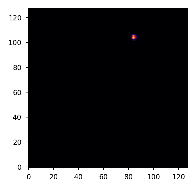
Note

Notice the use of origin='lower' in the plot above. For an explanation, see the note here.

DispersiveTilt

The DispersiveTilt class can be used to represent any wavelength-depentent tilt. Examples include modeling chromatic aberrations, prisms, or diffraction gratings, just to name a few. With a dispersive tilt, light is dispersed along a path called a spectral trace. The location of a specific wavelength along this trace is determined by the dispersion function.

The basic geometry of spectral dispersion is illustrated in the figure below:

The spectral trace is parameterized by a polynomial of the form

\[y = a_n x^n + \cdots + a_2 x^2 + a_1 x + a_0\]

and should return units of meters on the focal plane provided an input in meters on the focal plane.

Similarly, the wavelength along the trace is parameterized by a polynomial of the form

\[\lambda = a_n d^n + \cdots + a_2 d^2 + a_1 d + a_0\]

and should return units of meters of wavelength provided an input distance along the spectral trace.

Lentil supports trace and dispersion functions with any arbitrary polynomial order. While a simple analytic solution exists for modeling first-order trace and/or dispersion, there is no general solution for higher order functions.

As a result, trace and/or dispersion polynomials with order > 1 are evaluated numerically. Although the effects are small, this approach impacts both the speed and precision of modeling grisms with higher order trace and/or dispersion functions. In cases where speed or accuracy are extremely important, a custom solution may be required.

Grism

Warning

Grism is deprecated and will be removed in a future version. Use DispersiveTilt instead.

A grism is a combination of a diffraction grating and a prism that creates a dispersed spectrum normal to the optical axis. This is in contrast to a single grating or prism, which creates a dispersed spectrum at some angle that deviates from the optical axis. Grisms are most commonly used to create dispersed spectra for slitless spectroscopy or to create interference fringes for dispersed fringe sensing.

Lentil’s Grism plane provides a straightforward mechanism for efficiently modeling a grism.