Overview#
Loupe is a Python library for defining and solving optimization problems by minimizing scalar cost functions.
Loupe was designed to be:
User friendly - provide a simple, consistent interface for common use cases. Loupe is generally compatible with Numpy arrays and where possible, Loupe mimics Numpy’s API so if you know how to use Numpy, you know how to use Loupe.
Fast - forward models are defined and manipulated dynamically. These operations are automatically tracked in a computational graph, making it possible to analytically compute gradients which can then be fed to an optimizer - greatly speeding up optimization convergence.
Easy to extend - the core function object is designed to be subclassed, making it very easy to develop and use new operations
Importing Loupe#
Every public function and class is available in Loupe’s root namespace. Loupe’s standard library can be imported as follows:
>>> import loupe
Quickstart#
Creating models#
Loupe’s main object is the array. It is an n-dimensional container
of homogeneous elements (elements of the same type). Loupe’s arrays can be
combined or operated on by any of Loupe’s functions. Here, we’ll construct a
simple 2-D basis set and create some sample data we’ll try to match in the next
section:
>>> import numpy as np
>>> import matplotlib.pyplot as plt
>>> import loupe
>>> basis = loupe.zernike_basis(np.ones((100, 100)), np.arange(2, 7))
>>> coeffs = np.array([1.5, -2.5, 3, -6, 4])
>>> data = np.einsum('ijk,i->jk', basis, coeffs)
>>> plt.imshow(data)
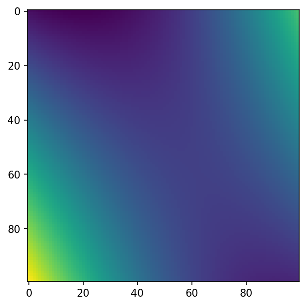
Now that we have some sample data, we’ll try to recover the coefficients used to create the data by defining a forward model and solving a simple optimization problem.
We need to define a Loupe array that will represent the parameter to be optimized. Since we don’t have a starting guess for the values, we’ll just set everything to zero:
>>> x = loupe.zeros(shape=5)
Next, we’ll define the forward model. This model multiplies the 2-D basis set by the
coefficients in x, and accumulates the result in a single 2-D array:
>>> model = loupe.einsum('ijk,i->jk', basis, x)
Optimizing the model parameters#
Loupe’s optimizer attempts to minimize any cost function that returns a scalar value. We’ll use a cost function that returns the sum squared error between the model and the data:
>>> cost = loupe.sserror(model, data, gain_bias_invariant=False)
We can now pass the cost function to the optimizer and ask it to solve for x:
>>> loupe.optimize(fun=cost, params=x)
     fun: array(2.53492193e-09)
hess_inv: <5x5 LbfgsInvHessProduct with dtype=float64>
     jac: array([ 2.35434693e-07, -3.92391155e-07,  5.46235343e-06, -9.22555260e-06,
       4.66570919e-06])
 message: 'CONVERGENCE: NORM_OF_PROJECTED_GRADIENT_<=_PGTOL'
    nfev: 7
     nit: 6
    njev: 7
  status: 0
 success: True
       x: array([ 1.50000743, -2.50001239,  3.00013613, -6.00028557,  4.00036117])
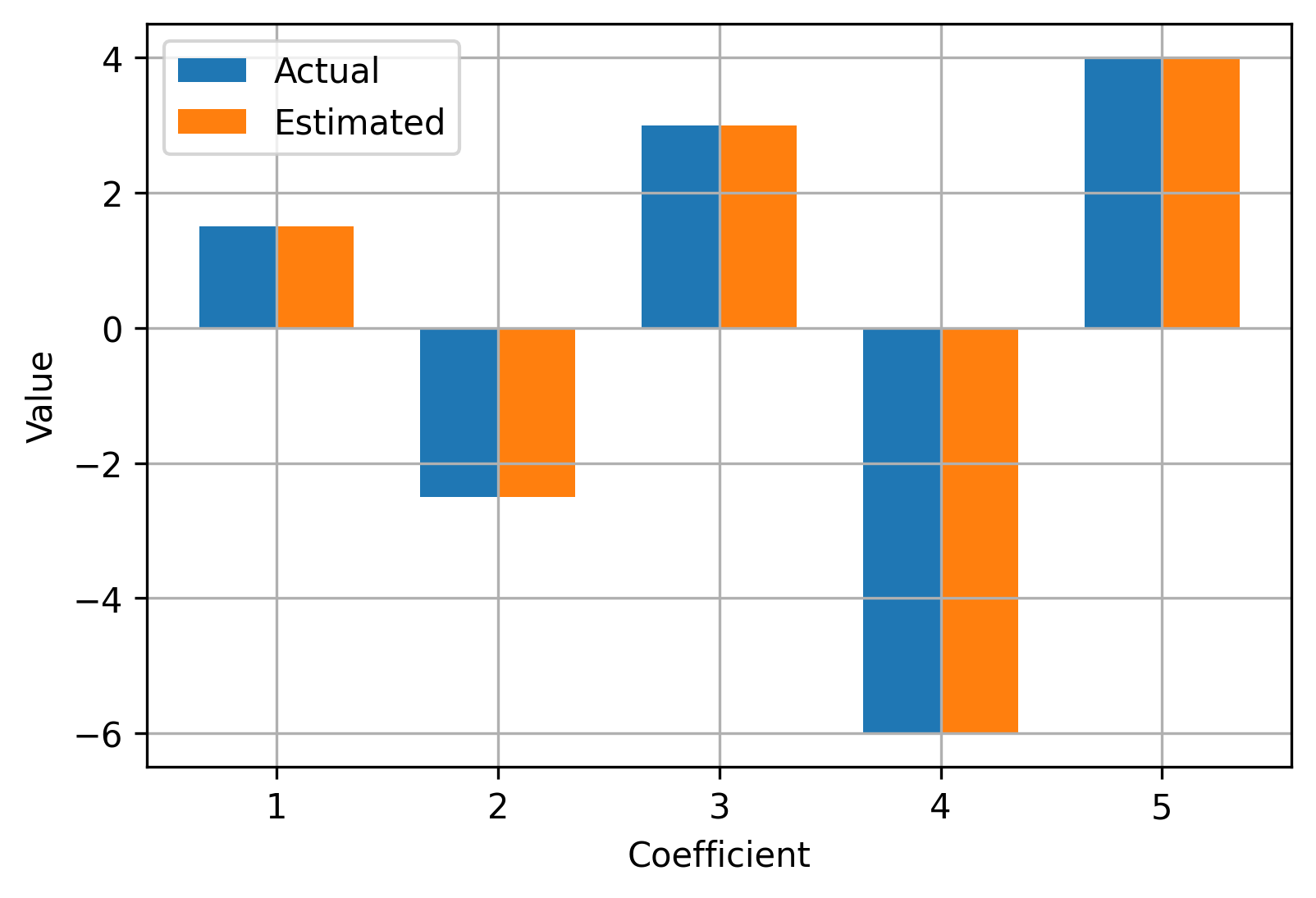
>>> print(coeffs - x)
[-7.4300e-06  1.2390e-05 -1.3613e-04  2.8557e-04 -3.6117e-04]
We see that the optimizer recovered values for x that are nearly identical to the
original values of coeffs that were used to generate the sample data. Great success!
Getting help#
The best place to ask for help on subjects not covered in this documentation or suggest new features/ideas is by opening a ticket on Github